Physics as Code: Why Foundation Models Fail Without First-Principles Constraints

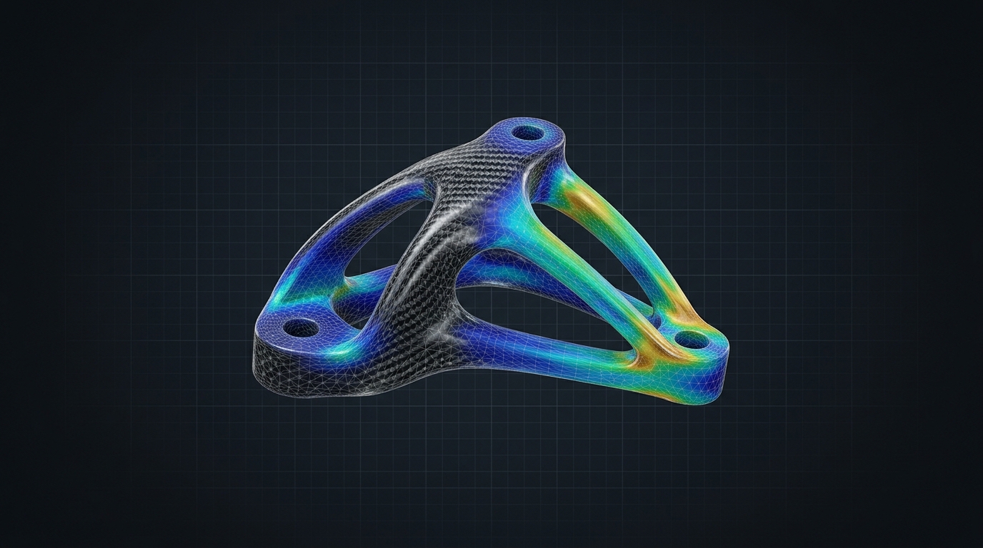
Language models are extraordinary at proposing ideas and completely illiterate at physics.

Ask a frontier model to design a 300-gram carbon fiber bicycle handlebar, plan an autoclave curing schedule, or calculate high-speed package spacing on a belt sorter. It will generate a confident, beautifully articulated plan. It will even give you realistic-sounding numbers.

Then you run that plan on the shop floor, and one of two things happens: the composite laminate delaminates in the mold due to exothermic resin runaway, or the packages collide on the divert spur because the acceleration ramps violated basic friction coefficients.

In software, a hallucination is an awkward sentence or a bad SQL join that gets caught in staging. In physical manufacturing, a hallucination is a ruined $40,000 aluminum compression mold, hundreds of meters of scrap pre-preg carbon fiber, or eight hours of emergency conveyor downtime.

Over twenty years of building carbon fiber components at Predator Cycling, industrial operating software at AyoWork, and sorting controls across enterprise distribution networks, I’ve learned a simple rule: never ask a probabilistic model to do a deterministic engine’s job.

[ PROBABILISTIC AGENT ] ──► [ DETERMINISTIC SOLVER ] ──► [ CLOSED-LOOP FEEDBACK ]
(Generates Candidate Part)   (FEA, Thermal, Kinematics)   (Typed Constraint Vectors)
          ▲                                                                 │
          └────────────────── REJECT / REFINE BOUNDARIES ───────────────────┘

---

Table of Contents

• The Hallucination Gap: Language vs. Mechanics
• Case 1: Thermal Expansion in Silicone-Intensified Molding
• Case 2: Orthotropic Anisotropy in Carbon Laminates
• The Solution: Physics as Code (The 3-Tier Stack)
• Closing the Loop: Typed Error Vectors
• Summary
• Technical Q&A

---

The Hallucination Gap: Language vs. Mechanics

A Large Language Model (LLM) predicts the next most likely token based on statistical correlations in text.

Text is full of human approximations. We write that “the part should be stiff and lightweight,” or that “we increased temperature gradually.” But physical materials do not care about grammar, marketing descriptions, or averages. Physical materials obey conservation of energy, Navier-Stokes fluid mechanics, and the laws of thermodynamics:

Dimension	Probabilistic Model (LLM)	Deterministic Physics Engine (FEA/CFD/CAD)
Output Type	Plausible token sequences	Numerically verified state vectors
Behavior	Interpolates between training texts	Solves boundary value differential equations
Edge Cases	Confidently hallucinates intermediate steps	Diverges, flags non-convergence, or rejects
Cost of Failure	Regenerate prompt ($0.002)	Broken tooling, scrap carbon, machine crash ($10k+)

If you want AI to solve real-world industrial problems, you cannot let the model operate directly on physical machines. You must enclose the model inside a hard boundary of first-principles mathematical constraints.

---

Case 1: Thermal Expansion in Silicone-Intensified Molding

Consider one of our proprietary manufacturing processes at Predator Cycling: silicone-intensified compression molding for hollow structural carbon components (such as our one-piece monolithic handlebars and bicycle dropouts).

In this process, pre-preg carbon plies are hand-laid into a CNC-machined 6061-T6 aluminum tool around a solid elastomeric silicone core. When the mold is bolted shut and heated inside an oven or heated platen press, the thermal expansion of the internal silicone generates intense hydrostatic consolidation pressure against the rigid aluminum walls, driving out interlaminar voids without needing a multi-million-dollar autoclave.

The governing physics is linear thermal expansion:

$\Delta L = \alpha \cdot L_0 \cdot \Delta T$

Where:

• $\alpha$ is the Coefficient of Thermal Expansion (CTE).
• $L_0$ is the initial dimension at ambient room temperature ($20^\circ\text{C}$).
• $\Delta T$ is the temperature delta to full resin cure ($135^\circ\text{C}$, $\Delta T = 115\text{ K}$).

Here is the physical catch:

$\alpha_{\text{silicone}} \approx 250 \times 10^{-6}\text{ K}^{-1}$

$\alpha_{\text{aluminum}} \approx 23 \times 10^{-6}\text{ K}^{-1}$

Silicone expands more than ten times faster than the aluminum mold cavity enclosing it.

If an AI design assistant sizes the silicone core based on room-temperature geometric cavity subtraction, one of two catastrophic physical failures will occur:

1. Core Over-Volume: If the core is 1.5mm too large at ambient temperature, the hydrostatic pressure at $135^\circ\text{C}$ will exceed 18 bar, stripping the tool’s grade-8 steel bolts, galling the aluminum parting line, and flashing resin across the shop floor.
2. Core Under-Volume: If the core is 1.0mm too small, thermal expansion will fail to bridge the internal volume delta before the epoxy resin reaches its gel point ($110^\circ\text{C}$). The laminate will cure with insufficient consolidation pressure ($P < 4\text{ bar}$), resulting in fatal interlaminar porosity and immediate structural rejection on the test bench.

An AI model cannot “feel” this thermal mismatch by reading text. But encode the CTE equations directly into the CAD parametric script, and the model literally cannot output an invalid core geometry.

---

Case 2: Orthotropic Anisotropy in Carbon Laminates

Steel and aluminum are isotropic materials. Their modulus of elasticity ($E$) and yield strength ($\sigma_y$) are identical in every spatial direction: $x$, $y$, and $z$.

Continuous fiber-reinforced composites are orthotropic. Unidirectional pre-preg carbon fiber (such as Toray T700 or T800 with 35% epoxy resin content) possesses immense tensile strength along the longitudinal fiber axis ($0^\circ$), but almost zero strength transverse to the fibers ($90^\circ$):

$E_{11} \approx 135\text{ GPa}, \quad E_{22} \approx 9.5\text{ GPa}$

$X_T \approx 2,400\text{ MPa}, \quad Y_T \approx 50\text{ MPa}$

The strength along the fiber is nearly fifty times greater than the strength across the resin matrix.

When human engineers or AI agents attempt to optimize a composite part purely for weight, they tend to orient fibers along the primary bending axis. But real-world structures experience complex multi-axial loading: torsional twisting, localized impact, and interlaminar peel forces at clamp junctions.

To predict failure in an orthotropic laminate, we must evaluate interactive failure criteria, such as the Tsai-Hill criterion:

$\frac{\sigma_1^2}{X^2} - \frac{\sigma_1 \sigma_2}{X^2} + \frac{\sigma_2^2}{Y^2} + \frac{\tau_{12}^2}{S^2} \ge 1.0$

Where $X$ is axial strength, $Y$ is transverse strength, and $S$ is in-plane shear strength.

If the value equals or exceeds $1.0$, the laminate fails. No amount of conversational prompt engineering can replace this tensor calculation. The software architecture must couple the generative agent to a headless FEA solver (such as Ansys or open-source CalculiX) that calculates the Tsai-Hill ratio across every ply in the laminate stack.

---

The Solution: Physics as Code (The 3-Tier Stack)

To harness the genuine speed and ideation capability of AI while maintaining zero scrap on the shop floor, we deploy a 3-tier architecture:

┌────────────────────────────────────────────────────────┐
│  TIER 1: PROBABILISTIC PROPOSER (AI Agent Swarm)       │
│  - Explores geometric design variations                │
│  - Optimizes weight, surface aerodynamics, ergonomics  │
│  - Proposes raw parametric CAD boundary constraints    │
└───────────────────────────┬────────────────────────────┘
                            │ Proposes candidate spec
                            ▼
┌────────────────────────────────────────────────────────┐
│  TIER 2: DETERMINISTIC PHYSICS SOLVER (The Gatekeeper) │
│  - Headless FEA & CFD mesh evaluation                  │
│  - Tsai-Hill / Hashin composite laminate failure check │
│  - CTE thermal mold expansion validation               │
│  - PLC conveyance kinematics & deceleration limits     │
└───────────────────────────┬────────────────────────────┘
                            │ Pass: Release to CAM
                            │ Fail: Return typed error contract
                            ▼
┌────────────────────────────────────────────────────────┐
│  TIER 3: CLOSED-LOOP ITERATION CONTROLLER              │
│  - Formats failure coordinates as structured JSON      │
│  - Updates agent memory with tested failure bounds     │
│  - Triggers localized parametric refinement            │
└────────────────────────────────────────────────────────┘

1. Tier 1: The Probabilistic Proposer

The AI agent is given a specific parametric envelope: rider fit coordinates (reach, drop, stack), clearance for internal hydraulic brake routing, and target mass. The model proposes adjustments to spline control points, head-tube transitions, and laminate ply schedules.

2. Tier 2: The Deterministic Solver

The candidate geometry is immediately converted into a structured mesh and evaluated against programmatic boundary conditions:

• Structural: 1,200 N out-of-saddle sprint load applied to the handlebar drops (ISO 4210 fatigue test standard).
• Thermal: Autoclave cure cycle heating ramp ($2^\circ\text{C}/\text{min}$ up to $135^\circ\text{C}$).
• Kinematics: Conveyor decelerations capped at $1.8\text{ m/s}^2$ to prevent package toppling.

3. Tier 3: The Closed Feedback Loop

If the solver passes all criteria with a safety factor $\text{SF} \ge 1.6$, the part is committed to the PDM/PLM database and queued for CAM toolpath generation.

If the solver rejects the candidate, it does not throw a generic error. It emits a typed, coordinate-specific failure contract.

---

Closing the Loop: Typed Error Vectors

The secret to making this architecture work is the format of the feedback returned to the model.

If you tell an agent “the part broke, try again”, the model will make random, uncoordinated guesses. But if you return a structured tensor vector, the agent refines its next candidate with remarkable precision:

{
  "status": "REJECTED",
  "failure_mode": "INTERLAMINAR_SHEAR_EXCEEDED",
  "location": {
    "x_mm": 142.5,
    "y_mm": -38.2,
    "z_mm": 88.0,
    "ply_index": 4,
    "nominal_orientation_deg": 0
  },
  "metrics": {
    "calculated_tsai_hill": 1.28,
    "allowable_limit": 1.00,
    "transverse_shear_stress_mpa": 64.2,
    "interlaminar_shear_strength_mpa": 50.0
  },
  "recommended_adjustment": "Add 45/-45 degree biaxial fabric patch between plies 3 and 5 to redistribute torsional shear."
}

When the agent receives this payload, it doesn’t hallucinate. It reads the exact spatial coordinates, understands the failure mechanism (transverse shear on $0^\circ$ unidirectional plies), and inserts a localized $\pm 45^\circ$ carbon twill reinforcement patch.

The solver runs again. Tsai-Hill drops to $0.78$. Safety factor verified. The loop closes deterministically.

---

Summary

1. Probabilistic models propose; deterministic engines verify. Never trust a generative language model to perform structural, thermal, or physical calculations.
2. Encode physics as immutable code boundaries. Thermal expansion coefficients ($\Delta L = \alpha L \Delta T$), laminate failure criteria, and kinematic limits belong in deterministic solvers, not in prompts.
3. Separate the proposer from the evaluator. The system that designs the geometry must never be the system that approves its structural integrity.
4. Feed failure vectors back to the agent. When a candidate fails, return structured coordinate and tensor data so the model can iterate with mathematical discipline.

When you bridge computational AI with the unforgiving laws of physical mechanics, you don’t just generate digital renders—you build hardware that endures.

---

Technical Q&A

Q: Why not fine-tune an LLM directly on FEA simulation data?

A: You can fine-tune models to predict approximate stress concentrations or suggest initial design seeds (surrogate modeling). However, surrogate models are still statistical approximations. In aerospace, automotive, or medical applications, a 2% statistical error can result in catastrophic failure. A deterministic solver running on finite element equations remains non-negotiable for final structural certification.

Q: How computationally expensive is this loop?

A: By using hierarchical meshing:

1. Fast coarse-mesh linear FEA runs in under 3 seconds to catch glaring structural defects.
2. Only candidates that pass coarse checks advance to non-linear, fine-mesh multi-physics evaluation (taking 2 to 5 minutes). Over 85% of bad candidates are rejected in the first 3 seconds, keeping compute costs minimal.

---

Related Deep Dives

• The Replayable Factory: Turning PLC Data into a Digital Twin That Can Rewind
• Agents Don’t Need More Autonomy. They Need a Gateway and a Memory
• The 5D Manufacturing Methodology