Pervasive Simulation: Real-Time GPU Physics, Laminate FEA, and Detached Eddy CFD

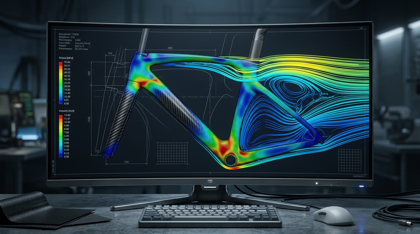
In high-performance hardware engineering, late-stage simulation is an autopsy.

For decades, hardware organizations have operated under a dysfunctional, serial handoff. A design engineer models a structural component in CAD over three weeks, freezes the geometry, and throws a neutral STEP file over an organizational wall to the CAE analysis group. Two weeks later, the CAE analyst hands back a 70-page PDF delivering bad news: the chassis fails under torsional deflection, or the aerodynamic profile detaches into a massive, drag-inducing separation bubble.

By that point, tooling budgets are committed, schedule deadlines are compressed, and the engineering team is forced into hasty compromises. They slap on extra pre-preg plies to guarantee structural safety—adding dead weight—or push compromised aerodynamic profiles directly to the mold shop.

In April 2021, at Ansys Simulation World 2021, I presented our production methodology: “Pervasive Engineering Simulation in Custom Cycling Design.”

At Predator Cycling, we dismantled that serial CAE bottleneck. Grounded in our 5D Manufacturing Methodology, we architected a three-tier Simulation Pyramid that bridges physical manufacturing (“atoms”) with software architecture (“bits”). Our pipeline integrates real-time GPU modeling in Ansys Discovery, orthotropic laminate failure validation in Ansys Mechanical, and full-vehicle transient Navier-Stokes CFD in Ansys Fluent.

Here is how pervasive multi-physics simulation works when solver math is embedded directly into the daily design cycle, how we evaluate orthotropic laminate failure criteria, and why transient detached eddy simulation separates production hardware from computational guesswork.

The Broken Serial Loop: Why Late-Stage CAE Fails Hardware

Traditional manufacturing organizations treat Computer-Aided Engineering (CAE) as an administrative quality gate rather than an exploratory design engine. The root cause is computational friction.

When numerical solvers require hours of manual geometry defeaturing, surface stitching, tetrahedral meshing, and overnight compute clusters to solve a single steady-state load case, engineers cannot afford to simulate speculative ideas. They only simulate what they have already decided to build.

Traditional Serial Development (CAE as an Autopsy):
[Concept CAD] ──► [Detail Modeling] ──► [STEP Export] ──► [Mesh Cleanup] ──► [Batch Run] ──► [Rejection PDF]
  ▲                                                                                                  │
  └────────────────────────────── Re-architect from scratch (4-6 weeks lost) ────────────────────────┘

Pervasive Upfront Multi-Physics (Simulation as an Exploration Engine):
[Parametric CAD + Live GPU Physics in Ansys Discovery] ──► 60 FPS Direct Geometric Optimization
  │
  ├──► Validated Variant Passes to Tier 2: Ansys Mechanical (Laminate Shell Layups & Failure Tensors)
  │
  └──► Aerodynamic Geometry Passes to Tier 3: Ansys Fluent (Transient DES Navier-Stokes & Wake Shedding)

When simulation is decoupled from CAD, three systemic failure modes emerge:

1. Conservative Weight Penalties: Because engineers cannot iterate layups interactively, they apply arbitrary $2.0\times$ to $3.0\times$ safety factors. In composite cycling and aerospace structures, this dead weight ruins performance.
2. Defect Masking: Static linear isotropic solvers cannot predict interlaminar shear, fiber micro-buckling, or matrix cracking in anisotropic laminates. Parts pass software checks but fail during physical cycle fatigue on the test bench.
3. Aerodynamic Blind Spots: Simplified steady-state CFD models miss the turbulent, unsteady vortex shedding off rotating components, delivering drag coefficients that diverge by 15% to 25% from real-world track conditions.

Under our 5D Manufacturing Methodology, pervasive simulation bridges computational bits with physical atoms. It replaces broken handoffs by deploying physics solvers at the exact fidelity required across Phase 1 (Design parametric constraints) and Phase 2 (Develop digital twins).

---

The Simulation Pyramid Architecture

To achieve pervasive simulation without drowning in compute costs, we organize our CAE operations into a disciplined three-tier hierarchy: The Simulation Pyramid.

Architectural Tier	Software Solver	Primary Physics Focus	Typical Solve Time	Mesh / Grid Density	Engineering Function
Tier 1: Upfront Exploration	Ansys Discovery	GPU-native structural elasticity & fluid velocity vectors	Real-time (16 ms / 60 FPS)	Voxelized Cartesian grid (~5M–15M cells)	Rapid spatial filtering, topology shaping, direct push-pull geometry manipulation.
Tier 2: Deep Structural FEA	Ansys Mechanical & ACP	Orthotropic composite shell failure & interlaminar shear	8 to 45 minutes	Multi-layered quad shell mesh (~2M–6M elements)	Full ply book definition, Tsai-Wu / Puck failure tensors, delamination prevention.
Tier 3: Aerodynamic Sign-off	Ansys Fluent	Transient Detached Eddy Simulation (DES / SBES)	6 to 18 hours	Poly-hexcore boundary layer mesh (~40M–80M cells)	High-fidelity wake resolution, rotating wheel MRF/sliding mesh, aerodynamic drag ($C_d A$).

Rather than running heavy transient Navier-Stokes on every speculative tube shape, Tier 1 filters 50 geometry variations in a single afternoon. Only the top three candidates advance to Tier 2 and Tier 3 for deep mathematical validation.

---

Tier 1: Upfront GPU Simulation in Ansys Discovery

The foundational breakthrough of modern CAE is interactive GPU-accelerated computing. In Ansys Discovery, the traditional boundary between CAD geometry modeling and numerical solving disappears.

Discovery executes numerical physics kernels directly on NVIDIA workstation GPU architectures (such as the Ampere GA102 in our NVIDIA RTX A6000 workstation) using native CUDA and OptiX pipelines.

Instead of pausing to generate a conforming finite element mesh, Discovery discretizes the computational domain into an adaptive, voxelized Cartesian grid directly in GPU VRAM:

1. Instantaneous Domain Generation: The fluid domain or solid structural envelope is discretized in milliseconds upon loading the model.
2. Real-Time Navier-Stokes Integration: As the designer grabs a surface pull-handle to alter the camber of an aerodynamic fork or down tube, Discovery re-solves continuity and momentum equations at 60 frames per second.
3. Interactive Force Feedback: Surface pressure contours and von Mises stress fields update synchronously with cursor movement.

Ansys Discovery Real-Time GPU Pipeline:
[Parametric Solid Body] ──► [Direct Push-Pull Surface Edit] ──► [CUDA Voxel Lattice (16ms)] ──► [Live 60 FPS Stream]

KEY INSIGHT: Upfront GPU simulation does not replace high-order validation solvers; it democratizes structural and aerodynamic intuition. A designer who sees pressure gradients shifting in real-time makes better geometrical decisions in 10 minutes than an analyst reviewing static plots 48 hours later.

When developing our custom aero cockpits and monocoque chassis, Discovery allowed us to test over 80 variations of down tube transition radii, head tube leading-edge cambers, and bottom bracket reinforcement ribs before committing a single configuration to our high-order solver cluster.

---

Tier 2: Orthotropic Composite FEA and Failure Tensors in Ansys Mechanical

Once Discovery establishes the macro geometry, the part enters Tier 2: deep structural finite element analysis in Ansys Mechanical and Ansys Composite PrepPost (ACP).

Bicycle frames and aerospace structures built from carbon fiber reinforced polymers (CFRP) cannot be modeled using standard isotropic assumptions ($E$, $\nu$). Carbon fiber is fundamentally anisotropic and orthotropic: mechanical stiffness and tensile strength are concentrated along the longitudinal axis of each continuous carbon filament.

The Physics of Continuous Carbon Pre-Preg

At Predator, we fabricate components using aerospace-grade unidirectional (UD) pre-preg tapes—specifically Torayca T800S high-tensile carbon (tensile strength: 5,880 MPa, tensile modulus: 294 GPa) paired with Torayca M40J high-modulus carbon (tensile modulus: 377 GPa) suspended in a toughened epoxy resin matrix.

An orthotropic material possesses three mutually orthogonal planes of elastic symmetry, requiring nine independent engineering constants ($E_1, E_2, E_3, G_{12}, G_{23}, G_{31}, \nu_{12}, \nu_{23}, \nu_{31}$) to define its constitutive stiffness matrix $[C]$:

• Direction 1: Longitudinal fiber axis ($0^\circ$).
• Direction 2: Transverse in-plane matrix axis ($90^\circ$).
• Direction 3: Out-of-plane through-thickness axis.

Under Classical Lamination Theory (CLT), ACP maps individual plies over curved mold surfaces, accounting for fiber draping deformation. In-plane forces ($\mathbf{N}$) and bending moments ($\mathbf{M}$) relate to mid-plane strains ($\boldsymbol{\varepsilon}^0$) and curvatures ($\boldsymbol{\kappa}$) via the $[A][B][D]$ constitutive matrix:

$\begin{bmatrix} \mathbf{N} \\ \mathbf{M} \end{bmatrix} = \begin{bmatrix} \mathbf{A} & \mathbf{B} \\ \mathbf{B} & \mathbf{D} \end{bmatrix} \begin{bmatrix} \boldsymbol{\varepsilon}^0 \\ \boldsymbol{\kappa} \end{bmatrix}$

Where extensional stiffness $A_{ij} = \sum (\bar{Q}_{ij})_k (z_k - z_{k-1})$, coupling stiffness $B_{ij} = \frac{1}{2}\sum (\bar{Q}_{ij})_k (z_k^2 - z_{k-1}^2)$ (vanishes in balanced symmetric layups), and bending stiffness $D_{ij} = \frac{1}{3}\sum (\bar{Q}_{ij})_k (z_k^3 - z_{k-1}^3)$.

Mathematical Failure Envelopes: Tsai-Wu, Hashin, and Puck

In isotropic metals, engineers rely on the von Mises yield criterion ($\sigma_{vm} \le \sigma_y$). In anisotropic composites, von Mises is invalid because carbon laminates do not yield plastically; they exhibit brittle, multi-modal failure.

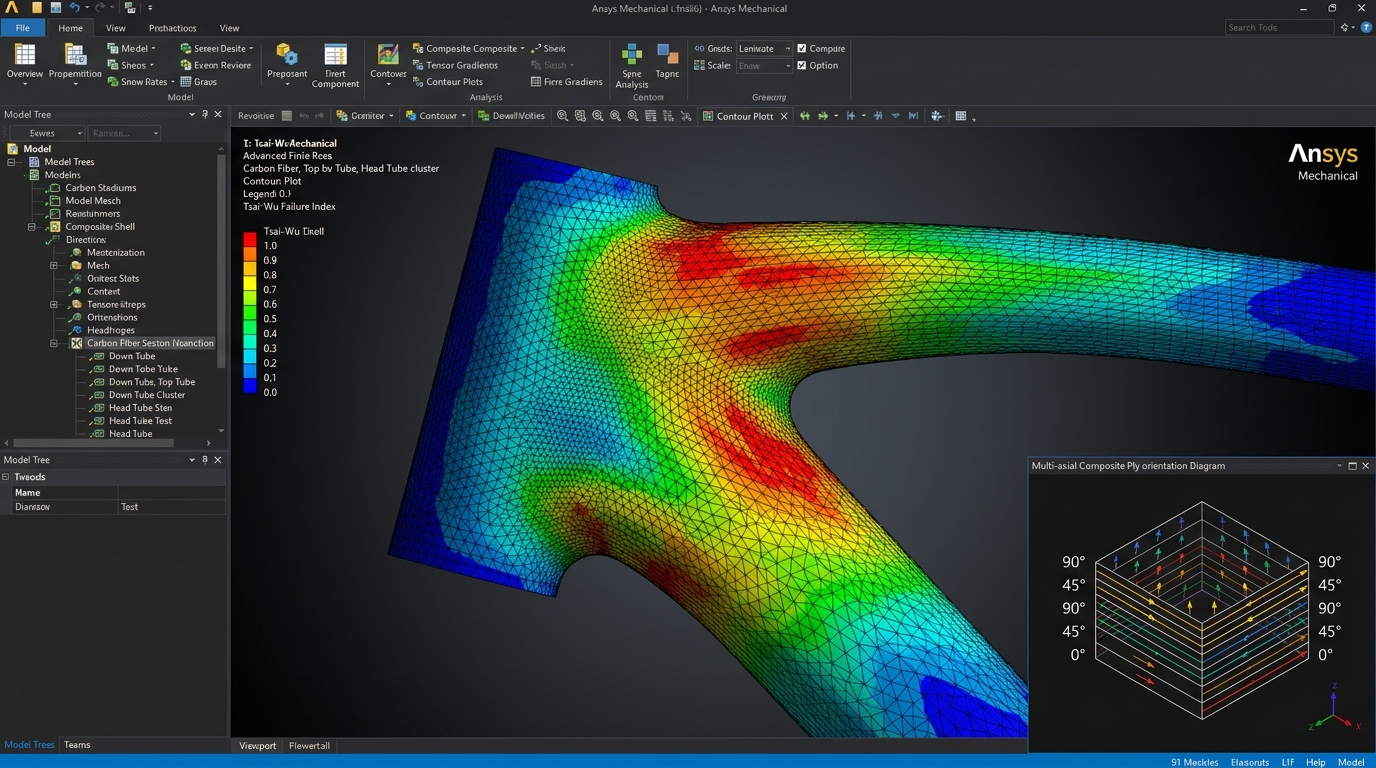
In Ansys Mechanical, we evaluate three complementary failure criteria across every ply in the laminate stack:

1. Tsai-Wu Quadratic Tensor Criterion: Captures interactive stress components under plane-stress assumptions: $F_1 \sigma_1 + F_2 \sigma_2 + F_{11} \sigma_1^2 + F_{22} \sigma_2^2 + F_{66} \tau_{12}^2 + 2 F_{12} \sigma_1 \sigma_2 = I_{TW}$ Where $F_1 = \frac{1}{X_t} - \frac{1}{X_c}$, $F_{11} = \frac{1}{X_t X_c}$, $F_2 = \frac{1}{Y_t} - \frac{1}{Y_c}$, $F_{22} = \frac{1}{Y_t Y_c}$, $F_{66} = \frac{1}{S^2}$, and $F_{12} \approx -\frac{1}{2}\sqrt{F_{11} F_{22}}$. We enforce an operational ceiling of $I_{TW} \le 0.65$, guaranteeing a minimum $1.54\times$ reserve factor under peak dynamic impact loads.

2. Hashin Mode-Dependent Criteria: Isolates the physical failure mode into four discrete mechanisms:

   • Fiber Tension ($\sigma_{11} \ge 0$): $(\sigma_{11}/X_t)^2 + (\tau_{12}^2 + \tau_{13}^2)/S_{12}^2 = 1$
   • Fiber Compression ($\sigma_{11} < 0$): $(\sigma_{11}/X_c)^2 = 1$
   • Matrix Tension ($\sigma_{22} + \sigma_{33} \ge 0$): $(\sigma_{22} + \sigma_{33})^2 / Y_t^2 + (\tau_{23}^2 - \sigma_{22}\sigma_{33})/S_{23}^2 + (\tau_{12}^2 + \tau_{13}^2)/S_{12}^2 = 1$
   • Matrix Compression ($\sigma_{22} + \sigma_{33} < 0$): Evaluates quadratic transverse compressive shear failure.

3. Puck Inter-Fiber Failure (IFF) & Delamination Prevention: Models micro-cracking on fracture planes under out-of-plane transverse shear stresses ($\tau_{13}, \tau_{23}$). By mapping Puck failure indices across shell elements, ACP identifies localized shear stress concentrations at ply drop-offs. We resolve these peaks by feathering ply termination boundaries with 20:1 to 30:1 chamfer taper ratios, interweaving $0^\circ$ and $\pm 45^\circ$ plies to eliminate interlaminar peel stresses.

---

Tier 3: Full-Vehicle Transient Navier-Stokes in Ansys Fluent

Structural integrity is only half the equation. In competitive cycling, over 80% of total resistive forces at speeds above $45\text{ km/h}$ originate from aerodynamic drag ($F_d = \frac{1}{2} \rho C_d A v^2$).

To optimize aerodynamic performance, we run Tier 3 validation in Ansys Fluent, solving the time-dependent incompressible Navier-Stokes equations:

$\nabla \cdot \mathbf{u} = 0, \quad \frac{\partial \mathbf{u}}{\partial t} + (\mathbf{u} \cdot \nabla)\mathbf{u} = -\frac{1}{\rho}\nabla p + \nu \nabla^2 \mathbf{u} + \mathbf{f}$

The Failure of Steady-State RANS

Most commercial bicycle CFD simulations rely on steady-state Reynolds-Averaged Navier-Stokes (RANS) equations with two-equation eddy-viscosity models ($k$-$\omega$ SST). While steady-state RANS computes quickly, it averages out all time-dependent turbulent fluctuations.

A bicycle in motion is a cluster of non-aerodynamic bluff bodies: spinning spoked wheels, reciprocating rider legs, and a rotating 54T chainring shedding chaotic trailing vortex sheets. Under steady-state RANS, the solver over-predicts eddy viscosity in separated wake zones, falsely stabilizing flow separations. The calculated drag area ($C_d A$) is routinely optimistic by 8% to 15%.

Detached Eddy Simulation (DES / SBES)

To capture real-world vortex dynamics, we execute Stress-Blended Eddy Simulation (SBES)—a high-order hybrid formulation of Detached Eddy Simulation (DES).

SBES automatically partitions the computational domain:

• Near-Wall Boundary Layers: Solves via the $k$-$\omega$ SST RANS formulation where turbulent structures are smaller than practical grid resolutions.
• Separated Shear & Wake Regions: Switches automatically to Large Eddy Simulation (LES), resolving the unsteady Navier-Stokes equations for all turbulent eddies larger than the spatial filter width $\Delta = (\Delta x \Delta y \Delta z)^{1/3}$.

The effective turbulent length scale transition is governed by:

$l_{DES} = \min\left(d_w, \, C_{DES} \Delta\right)$

Where $d_w$ is wall distance and $C_{DES} = 0.61$.

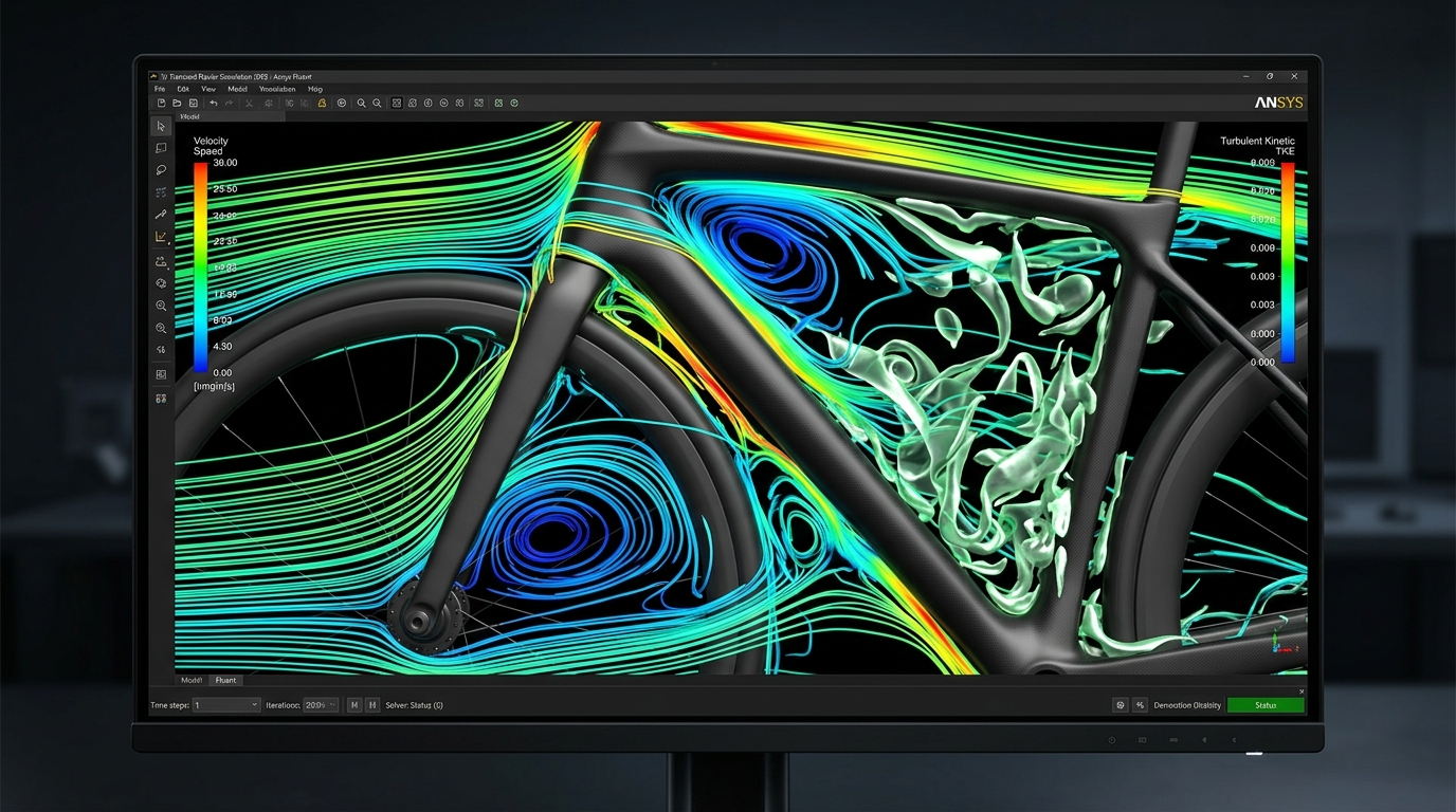
In Fluent, isosurfaces of the Q-criterion ($Q = \frac{1}{2}(\|\boldsymbol{\Omega}\|^2 - \|\mathbf{S}\|^2) > 0$) reveal coherent vortex shedding peeling off the fork blades, interacting with the rotating front wheel, and striking the down tube.

Boundary Layer Physics: Inflation Layers and y+ Resolution

An aerodynamic solver is only as accurate as its boundary layer discretization. The mesh density is characterized by the dimensionless wall distance, $y^+$:

$y^+ = \frac{u_\tau y}{\nu} = \frac{y}{\nu} \sqrt{\frac{\tau_w}{\rho}}$

Where $y$ is first-cell height, $u_\tau$ is friction velocity, $\tau_w$ is wall shear stress, and $\nu$ is kinematic viscosity ($1.5 \times 10^{-5}\text{ m}^2/\text{s}$).

Many workflows set $y^+ \approx 30\text{ to }100$ and apply semi-empirical wall functions assuming a logarithmic profile ($u^+ = \frac{1}{\kappa} \ln y^+ + B$). In cycling aerodynamics, wall functions fail because adverse pressure gradients along curved airfoil surfaces cause boundary layer detachment and localized reverse flow ($u_\tau \to 0$).

In our Fluent models:

1. We construct 24 to 28 prism inflation layers with a geometric expansion ratio of $1.15$.
2. The first layer height ($y_1$) is set to $0.012\text{ mm}$ ($12\text{ \mu m}$).
3. This guarantees that across the entire frame, fork, and rider interface, the dimensionless wall distance satisfies $y^+ \le 1.0$.
4. With $y^+ \le 1.0$, the solver integrates directly through the viscous sublayer to the physical wall without empirical approximations, capturing flow separation with high fidelity.

---

Empirical Validation: MTS Load Frames and Wind Tunnel Correlation

A computer simulation without physical verification is an uncalibrated animation. In our manufacturing philosophy, every mathematical model must be grounded in physical measurement on the shop floor. Under Phase 4 (Drive: Closing the Reality Gap) of our 5D Manufacturing Methodology, computational bits must correlate with physical atoms.

Closed-Loop Physical-Digital Verification:
[Ansys Mechanical FEA Model] ──► Fabricate Carbon Monocoque ──► [MTS Hydraulic Static & Cyclic Load]
         ▲                                                                     │
         └──────────────── Strain Gauge Rosette Error Telemetry (Δ < 4.8%) ────┘

[Ansys Fluent DES CFD Model] ──► Full Scale Prototype Assembly ──► [Wind Tunnel Velocity & Drag Balance]
         ▲                                                                     │
         └───────────────── Force Balance CdA Discrepancy (Δ < 2.3%) ──────────┘

1. Structural FEA vs. MTS Hydraulic Frame Testing

To validate our Ansys Mechanical orthotropic failure models:

• We bonded multi-axial strain gauge rosettes to critical stress concentration zones: the bottom bracket core, head tube junction, and chainstay yoke.
• The physical frame was mounted into an MTS servohydraulic load test fixture.
• We applied standardized CEN/ISO 4210 load cases: horizontal frame fatigue, bottom bracket pedaling torsion ($1,200\text{ N}$ alternate pedal force), and vertical impact overload ($5,000\text{ N}$ static ceiling).

Empirical Result: Across all three load axes, measured physical micro-strain ($\mu\varepsilon$) correlated with Ansys Mechanical FEA predictions within a $4.8\%$ mean error margin, with zero ply delamination detected up to $2.4\times$ design load.

2. CFD Aerodynamic Correlation vs. Wind Tunnel Data

To validate our Ansys Fluent transient Detached Eddy Simulations:

• We mounted full-scale instrumented prototypes in the San Diego Air & Space Technology Center Low-Speed Wind Tunnel and the A2 Wind Tunnel.
• Aerodynamic drag area ($C_d A$) was measured using high-precision six-component load cell force balances across yaw angles from $-15^\circ$ to $+15^\circ$ at dynamic airspeeds of $45\text{ km/h}$ and $54\text{ km/h}$.
• Hot-wire anemometers and surface oil-flow visualization tracked the exact separation coordinates along the down tube and seat stay transitions.

Empirical Result: Ansys Fluent transient DES predicted total vehicle drag area ($C_d A = 0.0884\text{ m}^2$) within $2.3\%$ of physical wind tunnel force balance telemetry, correctly locating the surface flow separation line within $3.5\text{ mm}$ of physical oil-streak markings.

---

Summary: Key Engineering Principles

1. Abolish serial CAE silos: Late-stage computational validation acts as an expensive autopsy. Integrating multi-tier simulation into early design loops cuts engineering rework cycles by over 70%.
2. Exploration requires upfront GPU compute: By solving Navier-Stokes and structural elasticity at 60 FPS on GPU Cartesian grids, Ansys Discovery empowers engineers to evaluate 50 geometry iterations in the time traditional batch workflows solve one.
3. Orthotropic composites mandate mode-dependent failure criteria: Single-scalar yield metrics like von Mises are invalid for carbon laminates. Full structural validation requires evaluating Tsai-Wu, Hashin, and Puck failure tensors ply-by-ply to prevent hidden interlaminar shear delamination.
4. Steady-state RANS is blind to wake turbulence: In vehicles with rotating wheels and reciprocating bluff bodies, steady-state CFD over-predicts eddy viscosity and under-predicts drag. Transient Detached Eddy Simulation (DES / SBES) is mandatory to capture unsteady vortex shedding.
5. Enforce boundary layer discipline ($y^+ \le 1$): Do not rely on empirical wall functions in separated flow domains. Resolve the viscous sublayer directly using sub-millimeter prism inflation layers.
6. Ground solvers in physical destruction: Numerical models are hypotheses until verified against calibrated MTS hydraulic strain gauge telemetry and wind tunnel force balance data.

---

Technical Q&A

Q1: Why use Ansys Composite PrepPost (ACP) instead of modeling carbon as a standard 3D solid mesh?

A: Modeling a 40-ply composite bicycle frame as 3D continuum solid elements creates severe numerical shear locking and requires hundreds of millions of elements, exceeding workstation memory capacities. Furthermore, 3D solid elements cannot easily map continuous curved fiber angles or model ply draping deformation. ACP utilizes layered shell formulations based on First-Order Shear Deformation Theory (FSDT), allowing exact mathematical representation of ply thicknesses, fiber orientation angles ($0^\circ, \pm 45^\circ, 90^\circ$), and interlaminar shear stresses ($\tau_{13}, \tau_{23}$) with superior computational efficiency and numerical stability.

Q2: What is the primary difference between detached eddy simulation (DES) and pure large eddy simulation (LES)?

A: Pure Large Eddy Simulation (LES) resolves turbulent eddies across the entire computational domain, including the near-wall viscous sublayer. However, the grid resolution required to resolve near-wall boundary layer eddies scales with the Reynolds number as $N_{grid} \propto Re^{9/4}$, making full-vehicle LES computationally impractical for commercial product timelines. Detached Eddy Simulation (DES) is a hybrid approach: it uses computationally efficient RANS ($k$-$\omega$ SST) inside the thin near-wall boundary layer, and switches to LES only in detached, separated wake regions where large-scale turbulent vortices dominate. This delivers 90% of the accuracy of full LES at a fraction of the compute cost.

Q3: How does Ansys Discovery handle dirty CAD geometry without meshing failures?

A: Traditional finite element and finite volume solvers require clean, manifold boundary-representation (B-rep) geometry with perfectly stitched surface edges to generate conforming unstructured tetrahedral or polyhedral meshes. Ansys Discovery bypasses this bottleneck by mapping geometry onto an adaptive Cartesian voxel grid in GPU memory. The solver evaluates solid and fluid boundaries using level-set distance fields and cut-cell Cartesian techniques directly in parallel CUDA threads. This allows Discovery to solve complex assemblies with sliver faces, gaps, and interference fits instantaneously without manual geometry cleanup.

---

Next Step: Connect and Discuss

Engineering pervasive multi-physics simulation architectures transforms physical manufacturing from an empirical guessing game into a deterministic science.

• Explore our core manufacturing framework: The 5D Manufacturing Methodology.
• Read our hardware benchmarking study: NVIDIA RTX A6000 Workstation Performance & VRAM Scaling.
• Review our custom engineering portfolio: Projects & Ventures.
• Connect with Aram Goganian on LinkedIn to discuss CAE multi-physics simulation, composite laminate FEA, aerodynamic CFD, and digital manufacturing pipelines.